The Line Blender: Optimizing Lineups Using MoneyPuck's Expected Goals Percentage (xG%)

Fire up the line blender. Over this series of posts, I'm going to explore an approach to finding optimal lineups using data-driven modeling. I'll start with the fundamentals of optimization before moving into more complex territory, using Graph Neural Networks (GNN) to evaluate previously unseen lines.

To begin, what's the difference between greedy and linear programming (LP) optimization?

Greedy optimization is straightforward: you pick the best available combination, then the next best, and so on. In other words, stack your lines, without considering the downstream effects on the rest of the roster. For most teams, this will create the best possible top line, but may leave the rest of the lineup wanting; or fail to provide a solution that fits the constraints of the problem (e.g., filling out all lines).

LP optimization, by contrast, identifies the best global solution by evaluating all possible line combinations. Instead of stacking top-heavy lines, LP can help find a lineup that maximizes team performance that meets problem constraints.

To see these ideas in action, I'll use MoneyPuck's expected goals percentage (xG%) limited to 5on5 play ¹. Optimizing for xG% is one way to choose an optimal lineup; at the end of the day, whoever scores more wins. Note that as a result of only looking at 5on5, the lineups do not explicity consider the value that players provide on special teams. Let's look at the Oilers' 2025-26 lineups as of Jan 25, 2026²:

• LP (>20 min. icetime)
• LP
• Greedy

LP optimization with a minimum icetime threshold: familiar lines emerge, some due to regress with more minutes played.

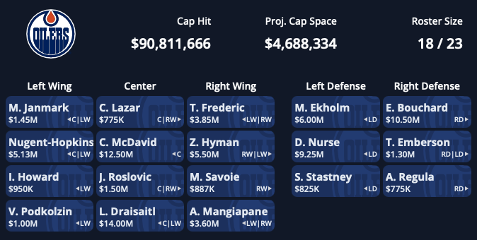
Forwards: Janmark, Lazar, Frederic (67% xG%); Nugent-Hopkins, McDavid, Hyman (64% xG%); Howard, Roslovic, Savoie (54% xG%); Draisaitl, Mangiapane, Podkolzin (53% xG%)
Defense: Ekholm, Bouchard (57% xG%); Nurse, Emberson (57% xG%); Regula, Stastney (44% xG%)

LP optimization produces four lines, but using this data, is dominated by lines with little icetime and high variance.

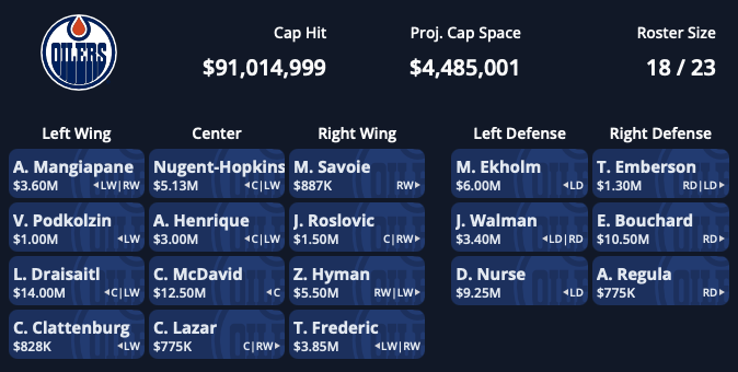
Forwards: Mangiapane, Nugent-Hopkins, Savoie (76% xG%); Podkolzin, Henrique, Roslovic (71% xG%); Draisaitl, McDavid, Hyman (70% xG%); Clattenburg, Lazar, Frederic (69% xG%)
Defense: Ekholm, Emberson (92% xG%); Walman, Bouchard (77% xG%); Nurse, Regula (52% xG%)

Greedy optimization fails to produce 4 valid forward lines.

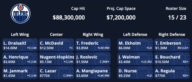
Forwards: Draisaitl, McDavid, Frederic (89% xG%); Henrique, Nugent-Hopkins, Roslovic (79% xG%); Janmark, Lazar, Mangiapane (44% xG%).
Defense: Ekholm, Emberson (92% xG%); Walman, Bouchard (77% xG%); Nurse, Regula (52% xG%)

---

One important thing to keep in mind when working with xG% and other performance measures is variance. In small samples, where lines or pairings have low icetime, results can swing wildly. One good or bad shift can swing the player's metrics. This high variance means we should be cautious about drawing strong conclusions from limited data.

Lineups also aren't optimized in a vacuum. Coaches often deploy their best lines against the opposition's best, and matchups can shift throughout a game. The "optimal" lineup on paper might not be the one that performs best in practice, especially when considering the need to adapt to different opponents and in-game situations. And ideally, lineups are more than just the sum of their parts. Players interact in ways that can amplify or diminish their individual contributions. The challenge is that there is limited icetime available to test every possible combination against real competition. So, how do we evaluate a combination that's never played together?

In my next post, we’ll move beyond historical data and use Graph Neural Networks (GNNs) to predict the performance of the unseen.

All posts in this series:
1. The Line Blender: Optimizing Lineups Using MoneyPuck's Expected Goals Percentage (xG%)
2. The Line Blender: Embedding Line Performance Using a GNN
3. The Line Blender: Using a GNN To Produce Olympic Rosters
4. The Line Blender: Using GNN Embeddings for Player Rankings
5. The Line Blender: Olympic Lineups with Announced Rosters
6. The Line Blender: Hypothetical Russian Olympic Lineups